Quantcast
Channel: BioCode's Notes
Viewing all 85 articles
Browse latest View live

My Formula as a Bioinformatician

$
0
0
Every day, I enjoy reading about bioinformatics in blogs, linkedin, and twitter; away from my daily reading of manuscripts journals. I strongly think that the future of publications/science will be closer & closer to the open access style and this emergent way to publish your ideas faster/brief in your own space. Some of my old co-workers don't understand this way to get in touch with science using informal environments rather than arbitrary/supervised spaces; I just said to them, we make the future, not the past. Reading the popular post “A guide for the lonely bioinformatician”, I was thinking about the last three years and how I have been built my own formula to survive as a lonely bioinformatician in a small country, with a lousy internet connection and without a bioinformatics environment.        

All the bioinformaticians that I met during these three years can be categorized in three major groups considering their original background:

1)    MDs, Biologist, Biochemist, Chemist
2)    Physicist, Mathematicians, Computer Scientist, Software Engineers, Software
       Developers
3)    Philosophers, *

As an embryonic and growing field the diversity is huge, then it is quite complex to express all the data behavior in one model or a formula. Here I will summarize some of the variables of my formula, extremely correlated with the original post suggestions:

1. Define yourself as The Bioinformatician

When I started to solve (mainly statistics and data handler) problems in my lab, all the PhD students and PostDocs addressed to me as the guy in charge of computational stuffs, the nerd of the team who can give you some statistics about your data quickly & nicely. In worst cases, I never hear again about the research conclusions or its future steps. After months, I decided to rename myself as the bioinformatician of the team and this step can be trivial but still important, you are not the Sys Admin, you are not the Developer, you are not the biologist with computational background, you are not the computer guy, you are not the excel guru, you are the BIOINFORMATICIAN
      
2. Learn as mush as possible from your lab questions

You can find two basic and orthogonal opinions: (i) those researchers who think is important to spend time in labs dealing with labs problems and the origin of the data & (ii) those researchers who think is not necessary at all. From my experience you should learn as much as possible from your lab without spending time in it. What I do: I participate from my lab discussions, invite lab co-workers for a coffee break and discuss and listen to their labs problems and the possible solutions; then I go back to my PC and read about it. As a bioinformatician you should care about the data itself, not how to obtain a better and quality data. 

Second issue is that you should spend time learning about how to detect data problems and inconsistencies, errors and finally perform the bioinformatics analysis. However, I like to be part of my lab team and I enjoy our technical discussions. As a bioinformatician they (and you) expect to propose integral solutions to your lab rather than partial answers to individual problems and questions. This topic is strongly related to with the first and the last suggestion of this post. Also you should learn from other labs questions and it is a good practice to accept manuscript revisions; starting from scratch (no-high impact journals). 
   
3. Learn batch and a Programming Language

Perhaps your lab is Windows oriented, but you shouldn’t be. Even if your daily work is in Windows, I can guaranty you, you are part of a 0.1% of the bioinformatics community. Unix/Linux is the chosen environment for bioinformatics and its key component is the command line interface. The term ‘shell’, or ‘UNIX shell’, refers to a command line interpreter for the UNIX/Linux operating system. Microsoft provides a command line interface for Windows, but this is not commonly used in bioinformatics. During these years I have worked on cheminformatics, proteomics and some genomics; in any of those fields command line skills are essential to handler data, submit your jobs to distributed systems, process big files, and interact with databases and services on internet. About a programming language, I will write some lines about it soon; meanwhile you can take a look to this pool. The most important thing is that you should be good enough to generate your own scripts, programs and at the end tools.      

4. Make friends with other bioinformatics groups.

As the original post says: “Develop electronic relationships with people and groups on the Internet. Develop a support group who will be able to help you with the kind of problems your lab-based group cannot”. This advice is crucial to grow as a bioinformatician or scientist in general and we are in a better position compare to other experimental fields. I normally use twitter, linkedin and skype to get in touch with my online co-workers and talk about data, programs and share ideas. I have more than 5 research manuscript with people that I have never met personally, but we have spent hours, sharing ideas, data and code. I posted in this Blog different lists with possible contacts in the field of Computational Proteomics and Bioinformatics.    

5. Develop your own research

If you arrive to this advice and use least 10% of the previous ones you will be able to start your own research. If you learn from the basic questions of your lab and you think about possible and complete solutions you are ready to generate your own questions, tools and studies. If you have the ideas, have also the tools to implement those ideas and have some contacts to learn and go faster in the right directions you will be able to conduct and develop your own research. If some of these ideas can be converted into manuscripts, it is a good practice to publish your own research apart from your common contributions to other papers in your lab.


From my point of view you can’t find the perfect model or formula, but you can learn as I did from different experiences and careers. I’m still learning.

Some References: 
  1 - So you want to be a computational biologist?
  2 - A guide for the lonely bioinformatician 
  3 - Collection of published “guides” for bioinformaticians 

Are you a Computational Biologist or Bioinformaticist or Bioinformatician?

$
0
0
A recent discussion was provoked by on twitter January 8 regarding what is the choice term for referring to those researchers working on Bioinformatics and Computational Biology fields.
This debate is older than people may think and it looks like an insignificant topic, but when you are writing your CV or your internet profile, or you’re looking for a new job, you will need a professional title, and that is really important. If you also look the volume of discussion and opinions about this topic on internet you will realize that the community have different points of view. I've use some of my spare time to read in detail different opinions about it, and also collect some those opinions and articles. Let’s see what common terms are used nowadays for these researchers:

Bioinformaticist, Bioinformatician, Computational Biologist, Digital biologist, bioinformatics analyst


In 2010 Grant Jacobs (@BioinfoTools) defined some of these categories in a post “More on ‘What is a computational biologist?’ (and related disciplines)”:

Computational biologist: Specialists, focusing on developing and applying theoretical biology.

Bioinformaticist: Generalists, developers/advanced users of informatics tools that manipulate biological data.

Digital biologist / bioinformatics analyst: Biologists who conduct bioinformatics analyses full-time, but don’t develop software (I prefer the latter term).

All of these terms are used in different context and situations; and this in fact tends to confuse young researchers in bioinformatics. The term Bioinformatician is commonly used in substitution of Bioinformaticist. From my point of view Digital biologist / bioinformatics analyst is almost never used and for that reason I will not comment in this post. 


Bioinformatician or Bioinformaticist:

Bioinformaticist had been replaced during recent years by Bioinformatician and some of the reasons can be found in different posts:

I think it has something to do with the termination of the word. Bioinformatics lends itself better to bioinformatician, just as mathematician sounds better than mathematicist. I would assume that fields ending in -tics (e.g. statistics) universally sound better with -tician, as it seems to be a more natural progression from the termination of the word.

 
I don't think there is a correct answer. For example, why do we say "mathematician", yet we say "physicist"?. I think most people choose which sounds better, to their ear. For me, that choice is "bioinformatician".


Bioinformaticist is an expert who not only knows how to use bioinformatics tools, but also knows how to write interfaces for effective use of the tools Bioinformatician on the other hand, is a trained individual who only knows to use bioinformatics tools without a deeper understanding.

Even when some people still use bionformaticist, as far as I can see, the term is obsolete and most of the bioinfo community members on internet (twitter, linkedin) dislike the old term. The Bioinformatician concept that is person, who only knows to use bioinformatics tools without a deeper understanding, looks more like a title for a bad bioinformatician rather than the current bioinformatician concept. From my point of view and what I see of how this term is currently used:

Bioinformatician: Bioinformatician tend to be generalists, computing skills can be applied across a fairly wide range of biological problems. Its nature does not require a deep biological knowledge, instead a bioinformatician also have known about fields such statistics and information theory. See also the post My formula as a Bioinformatician

Even Google suggest replacing the term Bioinformaticist by Bioinformatician.

Google suggestion for Bioinformaticist word.

 
Bioinformatician or Computational Biologist:

Some concepts about what is a computational biologist:

What characterizes computational biology (to me) is not a theoretical (read: basic) knowledge of biology, it is a knowledge of theoretical biology, a quite different (and more involved, detailed).

Computational biologists are leveraging specialist knowledge from particular areas generating results or developing tools that can be used by people outside those specialist areas (and in some cases, even experimental biologists within the same general niche).
 Grant Jacobs (@BioinfoTools)

The terms computational biology and bioinformatics are often used interchangeably. However, computational biology sometimes connotes the development of algorithms, mathematical models, and methods for statistical inference, while bioinformatics is more associated with the development of software tools, databases, and visualization methods.


But the community is mainly divided:


The below Google trends chart shows a comparison of How often both terms are searched:    


From my point of view a computational biologist is a BIOLOGIST researcher with computer science knowledge that can use this knowledge to generate software tools or new biological knowledge that can be used by people outside those specialist areas.

Bionformaticist is becoming extinct. Bioinformatician or Computational Biologist should be use depending of your environment, the position you are applying for (i.e. if you are applying for a Professor, PI or Group Leader position then is more often to use the term computational biologist boosting your contributions in biology using computational approaches; if you are to a daily working position where different fields of knowledge should be combine for the final results you should use the bioinfroamtician term). Another practical advice is to use the appropriate term considering the preferences of your group and your community. Bioinformatician is not a technical title as it is not statistician, or mathematician. More than 44 twitter users use the bioinformatician title compare with 26 computational biologist. It only boosts the informatics qualifications and skills.

What do you think?


Some of the most cited manuscripts in Proteomics and Computational Proteomics (2013)

$
0
0
Some of the most cited manuscripts in 2013 in the field of Proteomics and Computational Proteomics (no order):


     The PRoteomics IDEntifications (PRIDE, http://www.ebi.ac.uk/pride) database 
     at the European Bioinformatics Institute is one of the most prominent data 
     repositories of mass spectrometry (MS)-based proteomics data. Here, we 
     summarize recent developments in the PRIDE database and related tools. 
     First, we provide up-to-date statistics in data content, splitting the figures by 
     groups of organisms and species, including peptide and protein 
     identifications, and post-translational modifications. We then describe the 
     tools that are part of the PRIDE submission pipeline, especially the recently 
     developed PRIDE Converter 2 (new submission tool) and PRIDE Inspector 
     (visualization and analysis tool). We also give an update about the integration 
     of PRIDE with other MS proteomics resources in the context of the 
     ProteomeXchange consortium. Finally, we briefly review the quality control 
     efforts that are ongoing at present and outline our future plans.


     Next-generation sequencing allows the analysis of genomes, including those
     representing disease states. However, the causes of most disorders are 
     multifactorial, and systems-level approaches, including the analysis of 
     proteomes, are required for a more comprehensive understanding. The 
     proteome is extremely multifaceted owing to splicing and protein 
     modifications, and this is further amplified by the interconnectivity of proteins 
     into complexes and signalling networks that are highly divergent in time and 
     space. Proteome analysis heavily relies on mass spectrometry (MS). 
     MS-based proteomics is starting to mature and to deliver through a 
     combination of developments in instrumentation, sample preparation and 
     computational analysis. Here we describe this emerging next generation of 
     proteomics and highlight recent applications.
     SWATH-MS is a data-independent acquisition method that generates, in a 
     single measurement, a complete recording of the fragment ion spectra of all 
     the analytes in a biological sample for which the precursor ions are within a 
     predetermined m/z versus retention time window. To assess the performance 
     and suitability of SWATH-MS-based protein quantification for clinical use, we 
     compared SWATH-MS and SRM-MS-based quantification of N-linked 
     glycoproteins in human plasma, a commonly used sample for biomarker 
     discovery. Using dilution series of isotopically labeled heavy peptides 
     representing biomarker candidates, the LOQ of SWATH-MS was determined 
     to reach 0.0456 fmol at peptide level by targeted data analysis, which 
     corresponds to a concentration of 5–10 ng protein/mL in plasma, while SRM 
     reached a peptide LOQ of 0.0152 fmol. Moreover, the quantification of 
     endogenous glycoproteins using SWATH-MS showed a high degree of 
     reproducibility, with the mean CV of 14.90%, correlating well with SRM results 
     (R2 = 0.9784). Overall, SWATH-MS measurements showed a slightly lower 
     sensitivity and a comparable reproducibility to state-of-the-art SRM 
     measurements for targeted quantification of the N-glycosites in human 
     blood. However, a significantly larger number of peptides can be quantified 
     per analysis. We suggest that SWATH-MS analysis combined with 
     N-glycoproteome enrichment in plasma samples is a promising integrative 
     proteomic approach for biomarker discovery and verification.
       Phosphorylation, the reversible addition of a phosphate group to amino acid 
       side chains of proteins, is a fundamental regulator of protein activity, 
       stability, and molecular interactions. Most cellular processes, such as inter- 
       and intracellular signaling, protein synthesis, degradation, and apoptosis, 
       rely on phosphorylation. This PTM is thus involved in many diseases, 
       rendering localization and assessment of extent of phosphorylation of major 
       scientific interest. MS-based phosphoproteomics, which aims at describing 
       all phosphorylation sites in a specific type of cell, tissue, or organism, has 
       become the main technique for discovery and characterization of 
       phosphoproteins in a nonhypothesis driven fashion. In this review, we 
       describe methods for state-of-the-art MS-based analysis of protein 
       phosphorylation as well as the strategies employed in large-scale 
       phosphoproteomic experiments with focus on the various challenges and 
       limitations this field currently faces.

      Experience from different fields of life sciences suggests that accessible, 
      complete reference maps of the components of the system under study are 
      highly beneficial research tools. Examples of such maps include libraries of 
      the spectroscopic properties of molecules, or databases of drug structures in 
      analytical or forensic chemistry. Such maps, and methods to navigate them, 
      constitute reliable assays to probe any sample for the presence and amount 
      of molecules contained in the map. So far, attempts to generate such maps 
      for any proteome have failed to reach complete proteome coverage1, 2, 3. 
      Here we use a strategy based on high-throughput peptide synthesis and 
      mass spectrometry to generate an almost complete reference map (97% of 
      the genome-predicted proteins) of the Saccharomyces cerevisiae proteome. 
      We generated two versions of this mass-spectrometric map, one supporting 
      discovery-driven (shotgun)3, 4 and the other supporting hypothesis-driven 
      (targeted)5, 6 proteomic measurements. Together, the two versions of the 
      map constitute a complete set of proteomic assays to support most studies 
      performed with contemporary proteomic technologies. To show the utility of 
      the maps, we applied them to a protein quantitative trait locus (QTL) 
      analysis7, which requires precise measurement of the same set of peptides 
      over a large number of samples. Protein measurements over 78 S. 
      cerevisiae strains revealed a complex relationship between independent 
      genetic loci, influencing the levels of related proteins. Our results suggest 
      that selective pressure favours the acquisition of sets of polymorphisms that 
      adapt protein levels but also maintain the stoichiometry of functionally 
      related pathway members. 

     High-resolution mass spectrometry (MS)-based proteomics has progressed 
     tremendously over the years. For model organisms like yeast, we can now 
     quantify complete proteomes in just a few hours. Developments discussed in 
     this Perspective will soon enable complete proteome analysis of mammalian 
     cells, as well, with profound impact on biology and biomedicine.

       The complete extent to which the human genome is translated into 
       polypeptides is of fundamental importance. We report a peptidomic 
       strategy to detect short open reading frame (sORF)-encoded polypeptides 
       (SEPs) in human cells. We identify 90 SEPs, 86 of which are previously 
       uncharacterized, which is the largest number of human SEPs ever reported. 
       SEP abundances range from 10–1,000 molecules per cell, identical to 
       abundances of known proteins. SEPs arise from sORFs in noncoding RNAs as 
       well as multicistronic mRNAs, and many SEPs initiate with non-AUG start 
       codons, indicating that noncanonical translation may be more widespread in 
       mammals than previously thought. In addition, coding sORFs are present in 
       a small fraction (8 out of 1,866) of long intergenic noncoding RNAs.   
       Together, these results provide strong evidence that the human proteome is 
       more complex than previously appreciated.
      The landscape of human phosphorylation networks has not been 
      systematically explored, representing vast, unchartered territories within 
      cellular signaling networks. Although a large number of in vivo 
      phosphorylated residues have been identified by mass spectrometry 
     (MS)‐based approaches, assigning the upstream kinases to these residues 
      requires biochemical analysis of kinase‐substrate relationships (KSRs). Here, 
      we developed a new strategy, called CEASAR, based on functional protein 
      microarrays and bioinformatics to experimentally identify substrates for 289 
      unique kinases, resulting in 3656 high‐quality KSRs. We then generated 
      consensus phosphorylation motifs for each of the kinases and integrated this 
      information, along with information about in vivo phosphorylation sites 
      determined by MS, to construct a high‐resolution map of phosphorylation 
      networks that connects 230 kinases to 2591 in vivo phosphorylation sites in 
      652 substrates. The value of this data set is demonstrated through the 
      discovery of a new role for PKA downstream of Btk (Bruton's tyrosine kinase) 
      during B‐cell receptor signaling. Overall, these studies provide global insights 
      into kinase‐mediated signaling pathways and promise to advance our 
      understanding of cellular signaling processes in humans.
      Affinity purification coupled with mass spectrometry (AP-MS) is a widely used 
      approach for the identification of protein-protein interactions. However, for 
      any given protein of interest, determining which of the identified 
      polypeptides represent bona fide interactors versus those that are 
      background contaminants (for example, proteins that interact with the 
      solid-phase support, affinity reagent or epitope tag) is a challenging task. 
      The standard approach is to identify nonspecific interactions using one or 
      more negative-control purifications, but many small-scale AP-MS studies do 
      not capture a complete, accurate background protein set when available 
      controls are limited. Fortunately, negative controls are largely bait 
      independent. Hence, aggregating negative controls from multiple AP-MS 
      studies can increase coverage and improve the characterization of 
      background associated with a given experimental protocol. Here we present 
      the contaminant repository for affinity purification (the CRAPome) and 
      describe its use for scoring protein-protein interactions. The repository 
      (currently available for Homo sapiens and Saccharomyces cerevisiae)
      and computational tools are freely accessible at http://www.crapome.org/. 
       Several quantitative mass spectrometry based technologies have recently 
       evolved to interrogate the complexity, interconnectivity and dynamic nature 
       of proteomes. Currently, the most popular methods use either metabolic or 
       chemical isotope labeling with MS based quantification or chemical labeling 
       using isobaric tags with MS/MS based quantification. Here, we assess the 
       performance of three of the most popular approaches through systematic 
       independent large scale quantitative proteomics experiments, comparing 
       SILAC, dimethyl and TMT labeling strategies. Although all three methods 
       have their strengths and weaknesses, our data indicate that all three can 
       reach a similar depth in number of identified proteins using a classical (MS2 
       based) shotgun approach. TMT quantification using only MS2 is heavily 
       affected by co-isolation leading to compromised precision and accuracy. 
       This issue may be partly resolved by using an MS3 based acquisition; 
       however, at the cost of a significant reduction in number of proteins 
       quantified. Interestingly, SILAC and chemical labeling with MS based 
       quantification produce almost indistinguishable results, independent of   
       which database search algorithm used.
       Protein interaction topologies are critical determinants of biological function. 
       Large-scale or proteome-wide measurements of protein interaction 
       topologies in cells currently pose an unmet challenge that could
       dramatically improve understanding of complex biological systems. A 
       primary impediment includes direct protein topology and interaction 
       measurements from living systems since interactions that lack biological 
       significance may be introduced during cell lysis. Furthermore, many 
       biologically relevant protein interactions will likely not survive the 
       lysis/sample preparation and may only be measured with in vivo methods. 
       As a step toward meeting this challenge, a new mass spectrometry method 
       called Real-time Analysis for Cross-linked peptide Technology (ReACT) has 
       been developed that enables assignment of cross-linked peptides 
      “on-the-fly”. Using ReACT, 708 unique cross-linked (<5% FDR) peptide pairs 
       were identified from cross-linked E. coli cells. These data allow assembly of 
       the first protein interaction network that also contains topological features 
       of every interaction, as it existed in cells during cross-linker application. Of 
       the identified interprotein cross-linked peptide pairs, 40% are derived from 
       known interactions and provide new topological data that can help visualize 
       how these interactions exist in cells. Other identified cross-linked peptide 
       pairs are from proteins known to be involved within the same complex, but 
       yield newly discovered direct physical interactors. ReACT enables the first 
       view of these interactions inside cells, and the results acquired with this 
       method suggest cross-linking can play a major role in future efforts to map 
       the interactome in cells.
       To enhance therapeutic efficacy and reduce adverse effects of traditional 
       Chinese medicine (TCM), practitioners often prescribe a combination of 
       plant species and/or minerals called formulae. Unfortunately, the working 
       mechanisms of most of these compounds are difficult to determine and 
       thus remain unknown. In an attempt to address the benefits of formulae 
       based on current biomedical approaches, we analyzed the components of
       Yinchenhao Tang (YCHT), a classical formula and has been shown to be
       clinically effective for treating hepatic injury (HI) syndrome. The three
       principal components of YCHT are Artemisia annua L., Gardenia jasminoids
       Ellis, and Rheum Palmatum L., whose major active ingredients are 6,7 -
       dimethylesculetin (D), geniposide (G) and rhein (R), respectively. To 
       determine the mechanisms that underlie this formula, we conducted a
       systematic analysis of the therapeutic effects of the DGR compound using 
       immunohistochemistry, biochemistry, metabolomics and proteomics. Here, 
       we report that the DGR combination exerts a more robust therapeutic effect
      than any one or two of the three individual compounds by hitting multiple
      targets in a rat model of HI. Thus, DGR synergistically causes intensified
     dynamic changes in metabolic biomarkers, regulates molecular networks
     through target proteins, has a synergistic/additive effect and activates both
     intrinsic and extrinsic pathways.
 

What is a bioinformatician

$
0
0
By Anthony Fejes originally posted in blog.fejes.ca

I’ve been participating in an interesting conversation on linkedin, which has re-opened the age old question of what is a bioinformatician, which was inspired by a conversation on twitter, that was later blogged.  Hopefully I’ve gotten that chain down correctly.

In any case, it appears that there are two competing schools of thought.  One is that bioinformatician is a distinct entity, and the other is that it’s a vague term that embraces anyone and anything that has to do with either biology or computer science.  Frankly, I feel the second definition is a waste of a perfectly good word, despite being a commonly accepted method.


That leads me to the following two illustrations. How bioinformatics is often used, and I would argue that it’s being used incorrectly.:

bioinformatics_chart2

And how it should be used, according to me:

bioinformatics_chart1

I think the second clearly describes something that just isn’t captured otherwise. It covers a specific skill set that’s otherwise not captured by anything else. In fact, I have often argued that bioinformatician is really a position along a gradient from computer science to biology, where your skills in computer science would determine whether you’re a computational biologist (someone who applies computer programs to solve biology problems) or a bioinformatician (someone who designs computer programs to solve biology problems). Those, to me, are entirely different skill sets – and although bioinformaticians are often those who end up implementing the computer programs, that’s yet another skill, but can be done by a programmer who doesn’t understand the biology.

bioinformatics_chart3

That, effectively, makes bioinformatician an accurate description of a useful skill set – and further divides the murky field of “people who understand biology and use computers” – which is vague enough to include people who use an excel spreadsheets to curate bacterial strain collections. I suppose the next step is to get those who do taxonomy into the computational side of things and have them sort us all out.

Solving Invalid signature in JNLP

$
0
0
I have this error each time i run my jnlp:

invalid SHA1 signature file digest for

I found some discussions about possible solutions:

http://stackoverflow.com/questions/8176166/invalid-sha1-signature-file-digest

http://stackoverflow.com/questions/11673707/java-web-start-jar-signing-issue

But he problem was still there. I solved the problem using plugin option (<unsignAlreadySignedJars>true</unsignAlreadySignedJars>) and removing previous signatures to avoid possible signature duplications:


  <plugin>
     <groupId>org.codehaus.mojo.webstart</groupId>
       <artifactId>webstart-maven-plugin</artifactId>
         <executions>
           <execution>
             <id>jnlp-building</id>
             <phase>package</phase>
               <goals>
                 <goal>jnlp</goal>
               </goals>
            </execution>
        </executions>
         <configuration>
         <!-- Include all the dependencies -->
         <excludeTransitive>false</excludeTransitive>
         <unsignAlreadySignedJars>true</unsignAlreadySignedJars>
         <verbose>true</verbose>
         <verifyjar>true</verifyjar>
         <!-- The path where the libraries are stored -->
         <libPath>lib</libPath>
         <jnlp>
         <inputTemplate>webstart/jnlp-template.vm</inputTemplate>
          <outputFile>ProteoLimsViewer.jnlp</outputFile>
           <mainClass>cu.edu.cigb.biocomp.proteolims.gui.ProteoLimsViewer</mainClass>
         </jnlp>
         <sign>
           <keystore>keystorefile</keystore>
           <alias>proteolimsviewer</alias>
           <storepass>password</storepass>
           <keypass>password</keypass>
        <keystoreConfig>
            <delete>false</delete>
            <gen>false</gen>
          </keystoreConfig>
         </sign>
          <!-- building process -->
        <pack200>false</pack200>
         <verbose>true</verbose>
     </configuration>
     </plugin>

In the ERA of science communication, Why you need Twitter, Professional Blog and ImpactStory?

$
0
0
Where is the information? Where are the scientifically relevant results? Where are the good ideas? Are these things (only) in journals? I usually prefer to write about bioinformatics and how we should include, annotate and cite our bioinformatics tools inside research papers (The importance of Package Repositories for Science and Research, The problem of in-house tools); but this post represents my take on the future of scientific publications and their dissemination based on the manuscript “Beyond the paper” (1).

In the not too distant future, today’s science journals will be replaced by a set of decentralized, interoperable services that are built on a core infrastructure of open data and evolving standards — like the Internet itself. What the journal did in the past for a single article, the social media and internet resources are doing for the entire scholarly output. We are now immersed in a transition to another science communication system— one that will tap on Web technology to significantly improves dissemination. I prefer to represent the future of science communication by a block diagram where the four main components: (i) Data, (ii) Publications, (iii) Dissemination and (iv) Certification/Reward are completely interconnected:


Publications: The main paradigm of science communication during the last sixty years has been represented by the peer-review system, where editors and reviewers judge the scientific merit of submitted manuscripts on behalf of their communities. Currently, this traditional approach is changing due to the growing popularity of blog posts, videos and Preprints. From my point of view, some of the manuscript types usually hosted by traditional journals, such as Perspectives, Short Communications, and Technical Notes, are migrating to blogs posts, where they enjoy the benefits of open discussion and reader-driven rating systems without the meddling of god-like editors. In the last ten years the diversity of research outputs has increased dramatically, a dataset or a source code can be more appreciated by the community than their research manuscript. Then, we will increase in the near future the number of cites to datasets, code, opinions or blogs posts.

I don’t think the peer-review system will die, instead, it will be adapted to a more democratic and open environment where the community opinion will increase the credibility of the best results. At the same time, centralized systems or repositories (silos) will survive as well-curated and organized points of research data (papers, data, code).
  

Data: To interconnect and increase the publication system scope, researchers now share their data sets in repositories such as GenBank, ProteomeXChange and ArrayExpress. They use code repositories such as GitHub, CPAN, CRAN and GoogleCode to share code. figshare allows users to upload any kind of research data format (figures, datasets, media, papers, presentations) in a way that the current scholarly publishing model does not allow. Scientists are increasingly concerned with the reproducibility of their published results as well as the reusability of their data and code to draw new scientific conclusions.

Dissemination: The scholarly exchanges of academia are moving from classrooms, workshops and meetings to social media platforms such as Twitter, blogs, Facebook/LinkendIn Groups. As in other spheres of life, social media can simplify and expedite the dissemination of good manuscripts, tools, raw datasets or simply ideas. In a globally connected world where millions of people do science and millions of manuscripts are published every year, social digital networks facilitate the rapid communication of the best results and data, easing the access of the research community to opinion leaders and providing a nurturing environment for open discussions.     

Certifications/Reward: Peer-review will move into the open and become another public research product. The roles of the reviewer and editor will metamorphose from that of a gatekeeper to those of a collaborator, from an individual perspective to a community judgment. GoogleScholar’s citation system (where theses, web pages and preprints are also considered) ranks publications by relevance based on the number of citations, while ResearchGate’s download and citation numbers can be used as a measure of the acceptance of a manuscript by the community. The efforts of PubMed Commons are oriented to the retraction or endorsement of manuscript contributions. ImpactStory displays transparent and normalized metrics that reveal the diverse manners in which an article makes an impact.
          
The new ERA of science communication will claim scholarly products (blog posts, tweets, preprints, research papers, citations, data, code and presentation shares) rather than manuscripts. In the near future a research department will need more than good results or data for manuscripts or money to send members abroad to workshops and congress; they will need a complete system of twitter accounts, blogs or science media profiles to communicate its research. For researchers the advice follows a similar theme: it is becoming imperative to adapt and use those resources to be in touch with real-time science. In the future, science will be more open and decentralized, and we will jointly decide what the best ideas are, rather than having to believe blindly in Editors, Reviewers and Journals.

What do you think?


(1) Priem, J. (2013). Scholarship: Beyond the paper Nature, 495 (7442), 437-440 DOI: 10.1038/495437a

Most read from the Journal of Proteome Research for 2013.

$
0
0
1- Protein Digestion: An Overview of the Available Techniques and Recent
    Developments

    Linda Switzar, Martin Giera, Wilfried M. A. Niessen

    DOI: 10.1021/pr301201x

2-  Andromeda: A Peptide Search Engine Integrated into the MaxQuant
     Environment

     Jürgen Cox, Nadin Neuhauser, Annette Michalski, Richard A. Scheltema, Jesper
     V. Olsen, Matthias Mann

     DOI: 10.1021/pr101065j

2- Evaluation and Optimization of Mass Spectrometric Settings during
     Data-dependent Acquisition Mode: Focus on LTQ-Orbitrap Mass Analyzers
 
     Anastasia Kalli, Geoffrey T. Smith, Michael J. Sweredoski, Sonja Hess

     DOI: 10.1021/pr3011588

3-  An Automated Pipeline for High-Throughput Label-Free Quantitative
     Proteomics

     Hendrik Weisser, Sven Nahnsen, Jonas Grossmann, Lars Nilse, Andreas Quandt,
     Hendrik Brauer, Marc Sturm, Erhan Kenar, Oliver Kohlbacher, Ruedi Aebersold,
     Lars Malmström

     DOI: 10.1021/pr300992u

4-  Proteome Wide Purification and Identification of O-GlcNAc-Modified Proteins
     Using Click Chemistry and Mass Spectrometry

     Hannes Hahne, Nadine Sobotzki, Tamara Nyberg, Dominic Helm, Vladimir S.
     Borodkin, Daan M. F. van Aalten, Brian Agnew, Bernhard Kuster

     DOI: 10.1021/pr300967y

5-  A Proteomics Search Algorithm Specifically Designed for High-Resolution
     Tandem Mass Spectra

     Craig D. Wenger, Joshua J. Coon
   
     DOI: 10.1021/pr301024c

6- Analyzing Protein–Protein Interaction Networks

    Gavin C. K. W. Koh, Pablo Porras, Bruno Aranda, Henning Hermjakob, Sandra E.
    Orchard

    DOI: 10.1021/pr201211w

7-  Combination of FASP and StageTip-Based Fractionation Allows In-Depth
     Analysis of the Hippocampal Membrane Proteome

     Jacek R. Wisniewski, Alexandre Zougman, Matthias Mann

     DOI: 10.1021/pr900748n

8-  The Biology/Disease-driven Human Proteome Project (B/D-HPP): Enabling
     Protein Research for the Life Sciences Community

     Ruedi Aebersold, Gary D. Bader, Aled M. Edwards, Jennifer E. van Eyk, Martin
     Kussmann, Jun Qin, Gilbert S. Omenn

     DOI: 10.1021/pr301151m

 9-  Comparative Study of Targeted and Label-free Mass Spectrometry Methods
      for Protein Quantification

       Linda IJsselstijn, Marcel P. Stoop, Christoph Stingl, Peter A. E. Sillevis Smitt,
       Theo M. Luider, Lennard J. M. Dekker

       DOI: 10.1021/pr301221f

SWATH-MS and next-generation targeted proteomics

$
0
0
For proteomics, two main LC-MS/MS strategies have been used thus far. They have in common that the sample proteins are converted by proteolysis into peptides, which are then separated by (capillary) liquid chromatography. They differ in the mass spectrometric method used.

The first and most widely used strategy is known as shotgun proteomics or discovery proteomics. For this method, the MS instrument is operated in data-dependent acquisition (DDA) mode, where fragment ion (MS2) spectra for selected precursor ions detectable in a survey (MS1) scan are generated (Figure 1 - Discovery workflow). The resulting fragment ion spectra are then assigned to their corresponding peptide sequences by sequence database searching (See Open source libraries and frameworks for mass spectrometry based proteomics: A developer's perspective).

The second main strategy is referred to as targeted proteomics. There, the MS instrument is operated in selected reaction monitoring (SRM) (also called multiple reaction monitoring) mode (Figure 1 - Targeted Workflow). With this method, a sample is queried for the presence and quantity of a limited set of peptides that have to be specified prior to data acquisition. SRM does not require the explicit detection of the targeted precursors but proceeds by the acquisition, sequentially across the LC retention time domain, of predefined pairs of precursor and product ion masses, called transitions, several of which constitute a definitive assay for the detection of a peptide in a complex sample (See Targeted proteomics) .

Figure 1 - Discovery and Targeted proteomics workflows

Both methods have different and largely complementary preferred uses and performance profiles. Specifically, shotgun proteomics is the method of choice for discovering the maximal number of proteins from one or a few samples. In contrast, targeted proteomics is well suited for the reproducible detection and accurate quantification of sets of specific proteins in many samples as is the case in biomarker or systems biology studies.

At present, however, SRM is limited to the measurements of a few thousands transitions per LC-MS/MS run. To alleviate the limitations of the method, strategies have been developed that rely on neither detection nor knowledge of the precursor ions to trigger acquisition of fragment ion spectra. Those methods operate via unbiased “data-independent acquisition” (DIA), in the cyclic recording, throughout the LC time range, of consecutive survey scans and fragment ion spectra for all the precursors contained in predetermined isolation windows. Using such scans, the link between the fragment ions and the precursors from which they originate is lost, complicating the analysis of the acquired data sets. To date, the composite spectra generated by DIA methods have been principally analyzed with the standard database searching tools developed for DDA, either by searching the composite MS2 spectra directly or by searching pseudo MS2 spectra reconstituted postacquisition based on the co-elution profiles of precursor ions (from the survey scans) and of their potentially corresponding fragment ions.


"SWATH MS" is an alternative approach to proteome quantification that combines a high specificity DIA method with a novel targeted data extraction strategy to mine the resulting fragment ion data sets. The method uniquely combines a DIA methods with a innovative data analysis approach based on targeted data extraction developed in the Aebersold lab. Like in other DIA methods, the mass spectrometer cycles through precursor acquisition windows designed to cover the whole range of 400-1200 m/z - in which most of the proteotypic peptide precursors of an organism fall - within 2-4 seconds. During each cycle, the mass spectrometer will fragment all precursors from a given precursors window (e.g. 475 - 500 m/z for 25 Da windows) and record a complete, high accuracy fragment ion spectrum. The same range will be fragmented again in the next cycle, thus providing a time-resolved recording of fragment ions that elute on the chromatography. Thus the SWATH method provides highly multiplexed fragment ion spectra that are deterministically recorded over the complete chromatographic time.  The SWATH MS data analysis workflow consists of using a targeted data extraction strategy to query the acquired fragment ion maps for the presence and quantity of specific peptides of interest, using a priori information contained in spectral libraries.

The combination of high specificity fragment ion maps and targeted data analysis using information from spectral libraries of complete organisms offers unprecedented possibilities for the qualitative and quantitative probing of proteomes. 


If you are interested in the topic you can also read: 

- Gillet LC, Navarro P, Tate S, Röst H, Selevsek N, Reiter L, Bonner R, Aebersold R. Targeted data extraction of the MS/MS spectra generated by data-independent acquisition: a new concept for consistent and accurate proteome analysis. Mol Cell Proteomics. 2012 Jun;11(6):O111.016717. Epub 2012 Jan 18. PMID 22261725

 - Panchaud, A., A. Scherl, S. A. Shaffer, P. D. von Haller, H. D. Kulasekara, S. I. Miller, and D. R. Goodlett (2009, August). Precursor acquisition independent from ion count: how to dive deeper into the proteomics ocean. Analytical chemistry 81 (15), 6481-6488.

- OpenSWATH enables automated, targeted analysis of data-independent acquisition MS data Nat Biotech, Vol. 32, No. 3. (10 March 2014), pp. 219-223, doi:10.1038/nbt.2841 by Hannes L. Rost, George Rosenberger, Pedro Navarro, et al.

Java Optimization Tips (Memory, CPU Time and Code)

$
0
0

There are several common optimization techniques that apply regardless of the language being used. Some of these techniques, such as global register allocation, are sophisticated strategies to allocate machine resources (for example, CPU registers) and don't apply to Java bytecodes. We'll focus on the techniques that basically involve restructuring code and substituting equivalent operations within a method.  

EntrySet vs KeySet
-----------------------------------------

More efficient:

for (Map.Entry entry : map.entrySet()) {
Object key = entry.getKey();
Object value = entry.getValue();
}

than:

for (Object key : map.keySet()) {
Object value = map.get(key);
}


Avoid to create threads without run methods
------------------------------------

Usage Example:

public class Test
{
public void method() throws Exception
{
new Thread().start(); //VIOLATION
}
}
Should be written as:

public class Test
{
public void method(Runnable r) throws Exception
{
new Thread(r).start(); //FIXED
}
}

Initialise the ArrayList if you know in advance the size
--------------------------------------------

For example, use this code if you expect your ArrayList to store around 1000 objects:

List str = new ArrayList(1000)


Use ternary operators
----------------------------------------

class Use_ternary_operator_correction
{
public boolean test(String value)
{
if(value.equals("AppPerfect")) // VIOLATION
{
return true;
}
else
{
return false;
}
}
}

Should be written as:


class Use_ternary_operator_correction
{
public boolean test(String value)
{
return value.equals("AppPerfect"); // CORRECTION
}
}


Always declare constant fields Static

public class Always_declare_constant_field_static_violation
{
final int MAX = 1000; // VIOLATION
final String NAME = "Noname"; // VIOLATION
}

Should be written as:

public class Always_declare_constant_field_static_correction
{
static final int MAX = 1000; // CORRECTION
static final String NAME = "Noname"; // VIOLATION
}

Thesis: Development of computational methods for analysing proteomic data for genome annotation

$
0
0
Thesis by Markus Brosch in 2009 about Computational proteomics methods for analysing proteomic data for genome annotation.

Notes from Abstract

Proteomic mass spectrometry is a method that enables sequencing of gene product fragments, enabling the validation and refinement of existing gene annotation as well as the detection of novel protein coding regions. However, the application of proteomics data to genome annotation is hindered by the lack of suitable tools and methods to achieve automatic data processing and genome mapping at high accuracy and throughput. 

In the first part of this project I evaluate the scoring schemes of “Mascot”, which is a peptide identification software that is routinely used, for low and high mass accuracy data and show these to be not sufficiently accurate. I develop an alternative scoring method that provides more sensitive peptide identification specifically for high accuracy data, while allowing the user to fix the false discovery rate. Building upon this, I utilise the machine learning algorithm “Percolator” to further extend my Mascot scoring scheme with a large set of orthogonal scoring features that assess the quality of a peptide-spectrum match. 

To close the gap between high throughput peptide identification and large scale genome annotation analysis I introduce a proteogenomics pipeline. A comprehensive database is the central element of this pipeline, enabling the efficient mapping of known and predicted peptides to their genomic loci, each of which is associated with supplemental annotation information such as gene and transcript identifiers.

In the last part of my project the pipeline is applied to a large mouse MS dataset. I show the value and the level of coverage that can be achieved for validating genes and gene structures, while also highlighting the limitations of this technique. Moreover, I show where peptide identifications facilitated the correction of existing annotation, such as re-defining the translated regions or splice boundaries. 

Moreover, I propose a set of novel genes that are identified by the MS analysis pipeline with high confidence, but largely lack transcriptional or conservational evidence.


PepFinder™ Software: New Software Streamlines Protein Identification and Quantitation

$
0
0
PepFinder™ Software 

For biotherapeutic proteins to be effective, they must be produced in biologically active forms with proper folding and post-translation modifications (PTMs). Thermo Scientific™ PepFinder software provides accurate identification, in-depth characterization, and relative quantitation of biotherapeutic and other proteins from mass spectrometric data. It provides an automated workflows for glycopeptide identification, disulfide bond mapping, and quantification of PTMs. PepFinder software automates previously time-consuming manual processes, processing complex data and integrating the results into concise, informative reports. 

 - See more at: http://www.thermoscientific.com/content/tfs/en/product/pepfinder-software.html


ProteoStats: Computing false discovery rates in proteomics

$
0
0
By Amit K. Yadav (@theoneamit) & Yasset Perez-Riverol (@ypriverol):

Perl is a legacy language thought to be abstruse by many modern programmers. I’m passionate with the idea of not letting die a programming language such as Perl. Even when the language is used less in Computational Proteomics, it is still widely used in Bioinformatics. I’m enthusiastic writing about new open-source libraries in Perl that can be easily used. Two years ago, I wrote a post about InSilicoSpectro and how it can be used to study protein databases like I did in “In silico analysis of accurate proteomics, complemented by selective isolation of peptides”. 

Today’s post is about ProteoStats [1], a Perl library for False Discovery Rate (FDR) related calculations in proteomics studies. Some background for non-experts:

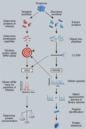
One of the central and most widely used approach for shotgun proteomics is the use of database search tools to assign spectra to peptides (called as Peptide Spectrum Matches or PSMs). To evaluate the quality of the assignments, these programs need to calculate/correct for population wise error rates to keep the number of false positives under control. In that sense, the best strategy to control the false positives is the target-decoy approach. Originally proposed by Elias & Gygi in 2007, the so-called classical FDR strategy or formula proposed involved a concatenated target-decoy (TD) database search for FDR estimation. This calculation is either done by the search engine or using scripts (in-house, non-published, not benchmarked, different implementations). 

So far, the only library developed to compute FDR at spectra level, peptide level and protein level FDRs is MAYU [2]. But, while MAYU only uses the classical FDR approach, ProteoStats provides options for 5 different strategies for calculating the FDR. The only prerequisite being that you need to search using a separate TD database as proposed by Kall et al (2008) [3]. Also, ProteoStats provides a programming interface that can read the native output from most widely used search tools and provide FDR related statistics. In case of tools not supported, pepXML, which has become a de facto standard output format, can be directly read along with tabular text based formats like TSV and CSV (or any other well-defined separator). 

Here, some concepts will be explained using the functions provided by the library. Let’s start:

A generic project starts from a database search, which can be done either with a (1) concatenated TD database (single search) or (2) separate T-D databases (two separate searches). Researchers then apply either Elias & Gygi formula (Concatenated) or Kall’s formula (Separate). 

FDR estimation formulae/methods in ProteoStats 

The ProteoStats library supports the following formulations on FDR estimation:

(1) Concatenated target decoy search based FDR [4], Concatenated FDR (FDRC)

This method was proposed by Elias and Gygi [4], although the basic concept of reverse database searching was based on Peng et al. [5] The database consists of combined set of proteins from target and their reversed sequences as decoy. In general, the ratio of false positives to true positives is estimated to be the FDR at the given threshold. The concatenated search is the most popular method of FDR estimation. The assumption is that for every decoy passing the threshold, there must be a corresponding false hit in target. Thus, the false positives are estimated by doubling the decoy count. The formula is-


(2) Simple/Separate target-decoy based FDR by Kall et. al [3], Separate/Simple FDR (FDRS)

This method was proposed by Kall et al as an alternative to combined search strategy. Kall et al suggested that combining the target and decoy databases overestimates the FDR and the decoy distribution no longer matches the target incorrect population. In this method, target and decoy searches are conducted separately. Each spectrum has one best target PSM and one best decoy PSM. Since the two searches are independent, it is assumed that the number of false positives amongst the targets is same as the number of decoys passing the threshold. It is also referred to as the simple FDR method by the authors. False positives are estimated by the count of decoys above the threshold. 


(3) Percentage of Incorrect target (PIT) correction to the above simple [3], FDR with PIT (FDRPIT)

Simple FDR described above assumes the size of true and false hits to be same or similar which is not an entirely correct assumption. Though all decoys contribute fully to the null distribution, all targets are not correct. Target distribution is a bimodal distribution representing the true and false target hits. This causes a non-balanced ratio of the true and false hits leading to overestimation of FDR. If a correction factor, Percentage of Incorrect Targets (PIT), is introduced in the equation 2 above, the FDR estimation is more accurate and increases sensitivity by allowing more correct hits at the same FDR. PIT is traditionally known as π0 or true negatives. This formulation depends on the percentage of incorrect target hits (PIT) that contribute to the negative (false) distribution as a weight in the above method to prevent overestimation of FDR and thus enhances the number of identifications. It should be noted that the name PIT is misleading since it is not a percentage but a fraction. 


(4) Refined formulation on Kall’s method [6], Refined Separate FDR (FDRRS)


In this formulation, the authors propose for calculating the FDR in the correct reference population by not doubling the estimated false targets by observing decoy hits above threshold directly. All decoys above threshold should not be taken as false positives unless they score more than target PSMs for the given spectrum. This simplification leads to inflation of decoy population and thus overestimation of FDR. The hits could be above threshold only in target (target only) or only in decoy (decoy only). When both are above threshold, either target could be better (target better) or the decoy (decoy better). Only decoy better are considered to be false positives and their count is doubled as suggested in Elias and Gygi method. The FDR in the correct reference population is then calculated by estimating the false positive PSM by subtracting from this population (decoy better + target better + target only), and dividing the result by the same number. The formula thus becomes- 


(5) Refined method on Elias et al method [7], FDRRC 

In this formulation, the authors argue that since decoy hits are obviously wrong, they can be disregarded in FDR estimation and thus the FDRRC formula is changed to yield the following formula-


ProteoStats supports these two methods and some of their alternate formulae described above, which provide better results. The newer formulae seem to work better but not much in practice due to code availability. It also follows that proteomics community has not settled for a single formula and these differ in basic concept. A primary testing of FDR method suited to a lab protocol is thus recommended. The five methods are explained in the paper. The details for installation, dependencies and developer documentation can be found in Documentation downloaded with the code. 

Quick Guide, Examples, Data & Results files 

Example Scripts Many example scripts are provided in the tests folder.

Data:

The files are provided in the DATA folder. Every file name is self-explanatory with a tag for target or decoy and algorithm name. For every algorithm, file names are like this-

QTOF_target_masswiz.csv 
QTOF_decoy_masswiz.csv

Results:

The example result files are provided in the OUTPUT folder.

File Parsers

Some inbuilt functions can be used to parse XML or native search engine files into tabular text (CSV/TSV) formats. For example X!Tandem XML, pepXML, Mascot dat etc.

FDR estimation

The user has two files per search after database search - one Target and one corresponding
Decoy file. Choose the script corresponding to the search algorithm used for database searching.


use MODULES::PSMFileIO; #file reading & parsing
use MODULES::PepXMLParser; #parsing pepXML files

#parse tandem XML file
my $tandemCSV = ReadTandemXML($tar); #Tandem target/decoy XML file

#parse Sequest XLS file from Thermo ProteomeDiscoverer
my $SequestCSV = ReadSequestXLS($tar); #Tandem target/decoy XML file

#parse pepXML file to TSV XLS file
my $pepXML2tsv = ReadPepXML($tar); #pepXML to TSV file
#parse Mascot dat file, convert to pepXML and parse the PepXML file
system("Mascot2XML $tar -notgz -nodta -D$tardb"); # convert to pepXML using  Mascot2XML from TPP

my $pepXML2tsv = ReadPepXML($tarpepXML); #pepXML to TSV file


Test_MassWiz.pl 
Test_Tandem.pl 
Test_OMSSA.pl 
Test_Mascot.pl
Test_Sequest.pl
Test_pepXML.pl 
Test_AnyText.pl

Edit any one of the script to enter the file names in @Tars, @Decs and @Outs arrays. Run the following command perl Test_MassWiz.pl and press enter to calculate FDR for input files. These scripts have a complete pipeline. 

Use Modules Examples

Initially, the program requires the use pragmas for calling specific modules from library. If you are writing your code in tests folder, you need to specify the base directory (ProteoStats, so that it can find MODULES folder) by use lib ‘../’ pragma.


use strict;
use warnings;
uselib '../'; #to define base directory
useMODULES::FDRCalculator; #main module that controls calling others
useMODULES::PSMFileIO; # Handles input file reading and Output writing
useMODULES::PepXMLParser; # Handles pepXML parsing
use MODULES::SeparateFDR; # Calculates FDRS
useMODULES::ConcatenatedFDR; # Calculates FDRC
useMODULES::FDRPIT; Calculates FDRPIT
useMODULES::RefinedConcatenatedFDR; Calculates FDRRC
useMODULES::RefinedSeparateFDR; Calculates FDRRS
use MODULES::ChartMaker; # Creates ScatterPlot, Histogram, ROC curves
use MODULES::ComparisonVenn; # Creates Venn, Compares PSMs/Peptides


Apart from the FDR and q-value calculations, ProteoStats can also be used for following tasks-

(1) Generating ROC curves

ROC curves can be plotted by the function ROCfromFDRFile.

use MODULES::ChartMaker; #
#define the parameters/arguments
my @FDRfiles = (‘FDR1_mascot.csv’,
                ‘FDR2_masswiz.csv’,
                ‘FDR3_omssa.csv’)#input files
my @seriesname = (‘Mascot’,‘MassWiz,‘OMSSA’)#corresponding seriesname
my $out = ‘MyROC.xlsx’ ; # Excel Output
my $FDRthr = 0.05; # FDR cutoff to show in ROC
my $qvalcol = -1; #column number for q-value. -1 means last column

#Call the ROC function with the arguments
$out=ROCfromFDRFile(\@FDRfiles,\@seriesname,$out,$FDRThr,$qvalcol);

exit;


(2) Generating Scatter Plots

Scatterplots can be generated using the function ScatterPlot_FDRFile.

use MODULES::ChartMaker; #
#define the parameters/arguments
my@FDRfiles = (‘FDR1_masswiz.csv’,
                ‘FDR2_masswiz.csv’,
                ‘FDR3_masswiz.csv’); #input files
my$xcol = 5;
my$xcolname = Mass’;
my$ycol = 7; #last column
my$ycolname = ‘Score’;
my $out = ‘MyScatter.xlsx’ ; #Excel Output

#Call the ScatterPlot function with the arguments
$out= ScatterPlot_FDRFile(\@FDRfiles,$xcol,$xcolname,$ycol,$ycolname,$out);

exit;


(3) Generating Histograms

Histograms can be generated using the function HistogramsfromFile function.

use MODULES::ChartMaker;

#define the input/arguments
my@files = (‘FDR_MassWiz1.csv’, FDR_ MassWiz2.csv’, FDR_ MassWiz3.csv’); #FDR Files
my$use_linear_axes = 1;
my$use_integral_bins= 0;

HistogramsfromFile(@files, @columns, $bins)


(4) Comparing FDR outputs and Creating Venn Diagrams 

This is a handy utility that can compare two or three FDR files. The FDR files need to contain only the filtered PSMs , else it will compare everything without any cutoff of score/p-value/e-value.

Start by defining the input files and Venn legends. Define 2 files for two set comparison and 3 for a three way comparison. Also define the column numbers for the FDR file for scans, peptide and protein columns.

useMODULES::ComparisonVenn;

#define the input/arguments
my$FDR1 = ‘FDR_MassWiz1.csv’; #FDR File 1
my$FDR2 = ‘FDR_ MassWiz2.csv’; #FDR File 2
my$FDR3 = ‘FDR_ MassWiz3.csv’; #FDR File 3
my$out = ‘Comparison_MassWiz_3_replicates.csv’; # OUTPUT File

# Define the labels for Venn
my$legend1 =‘MassWiz_rep1’;
my$legend2 =‘MassWiz_rep2’;
my$legend3 = ‘MassWiz_rep3’;

#Define column numbers for ScanID, peptide and Proteins
my$scancol = 0; #scan column
my$pepcol = 3; #peptide column

my$protcol = 7; #protein column

Read the files and get the data structures as hash references for easy comparison. Dereference the hashes.

#Get Hashrefs for Spectra and Peptides for comparison
my($SpecRef1,$PepRef1) = ReadSpecPep($FDR1,$scancol,$pepcol,$protcol);
my($SpecRef2,$PepRef2) = ReadSpecPep($FDR2,$scancol,$pepcol,$protcol);
my($SpecRef3,$PepRef3) = ReadSpecPep($FDR3,$scancol,$pepcol,$protcol);

#Dereference the hashrefs
my%SpecFDR1 = %$SpecRef1;
my%SpecFDR2 = %$SpecRef2;
my%SpecFDR3 = %$SpecRef3;
my%PepFDR1 = %$PepRef1;
my%PepFDR2 = %$PepRef2;

my%PepFDR3 = %$PepRef3;

Create Venn diagrams for 2 or 3 sets as per requirement. Define a title for chart and call the function CreateVenn2 or CreateVenn3 as shown in example below.

##Create Venn Charts for 3 or 2 sets passing spectra comparison
# Venn 3 sets ScanIDs
my$title1 = 'Spectra Comparison'; #Chart title
my$VennSpec3 = CreateVenn3 ([keys%SpecFDR1], [keys%SpecFDR2], [keys%SpecFDR3], $legend1, $legend2, $legend3, $title1, "$out.spectra.png" ) ;
print"Spectra venn created in file $VennSpec3\n";

#or try Venn 2 sets ScanIDs
my$VennSpec2=CreateVenn2( [ keys%SpecFDR1 ] , [ keys%SpecFDR2 ] , $legend1,$legend2,$title1,"$out.spectra.png") ;
print"Spectra venn created in file $VennSpec2\n";

##Create Venn Charts for 3 or 2 sets for peptide comparison
# Venn 3 sets peptides
my$title2 = 'Peptides Comparison';
my$VennPep3 = CreateVenn3([ keys%PepFDR1], [keys%PepFDR2], [keys%PepFDR3], $legend1, $legend2, $legend3, $title2, "$out.peptide.png" ) ;

print"Peptide venn created in file $VennPep3\n";


Finally, the comparisons can also be made and results written to a CSV file. The function CompareFDR3 or CompareFDR2 can be used with the hash references. The CSV file $out (defined in the input at the beginning of this code) contains the output of the comparisons. 

Reference List 

[1] Yadav, A. K.; Kadimi, P. K.; Kumar, D.; Dash, D. ProteoStats--a library for estimating false discovery rates in proteomics pipelines. Bioinformatics 2013, 29 (21), 2799-2800. 

[2] Reiter, L.; Claassen, M.; Schrimpf, S. P.; Jovanovic, M.; Schmidt, A.; Buhmann, J. M.; Hengartner, M. O.; Aebersold, R. Protein identification false discovery rates for very large proteomics data sets generated by tandem mass spectrometry. Mol. Cell Proteomics 2009, 8 (11), 2405-2417. 

[3] Kall, L.; Storey, J. D.; MacCoss, M. J.; Noble, W. S. Assigning significance to peptides identified by tandem mass spectrometry using decoy databases. J. Proteome. Res. 2008, 7 (1), 29-34. 

[4] Elias, J. E.; Gygi, S. P. Target-decoy search strategy for increased confidence in large-scale protein identifications by mass spectrometry. Nat. Methods 2007, 4 (3), 207-214. 

[5] Peng, J.; Elias, J. E.; Thoreen, C. C.; Licklider, L. J.; Gygi, S. P. Evaluation of multidimensional chromatography coupled with tandem mass spectrometry (LC/LC-MS/MS) for large-scale protein analysis: the yeast proteome. J. Proteome. Res. 2003, 2 (1), 43-50. 

[6] Navarro, P.; Vazquez, J. A refined method to calculate false discovery rates for peptide identification using decoy databases. J. Proteome. Res. 2009, 8 (4), 1792-1796. 

[7] Cerqueira, F. R.; Graber, A.; Schwikowski, B.; Baumgartner, C. MUDE: a new approach for optimizing sensitivity in the target-decoy search strategy for large-scale peptide/protein identification. J. Proteome Res. 2010, 9 (5), 2265-2277.

Making Your Code Citable

$
0
0
Original post from GitHub Guides:

Digital Object Identifiers (DOI) are the backbone of the academic reference and metrics system. If you’re a researcher writing software, this guide will show you how to make the work you share on GitHub citable by archiving one of your GitHub repositories and assigning a DOI with the data archiving tool Zenodo.
ProTip: This tutorial is aimed at researchers who want to cite GitHub repositories in academic literature. Provided you’ve already set up a GitHub repository, this tutorial can be completed without installing any special software. If you haven’t yet created a project on GitHub, start first byuploading your work to a repository.

 Choose your repository
Repositories are the most basic element of GitHub. They’re easiest to imagine as your project’s folder. The first step in creating a DOI is to select the repository you want to archive in Zenodo. To do so, head over to your profile and click the Repositories tab.
login
Important! Make sure you tell people how they can reuse your work by including a license in your repository. If you don’t know which license is right for you, then take a look at choosealicense.com.

Login to Zenodo

Next, head over to Zenodo and click the Sign In button at the top right of the page, which gives you an option to login with your GitHub account.
login
Zenodo will redirect you back to GitHub to ask for your permission to share your email address and the ability to configure webhooks on your repositories. Go ahead and click Authorize application to give Zenodo the permissions it needs.
auth

Pick the repository you want to archive

At this point, you’ve authorized Zenodo to configure the repository webhooks needed to allow for archiving and DOI-issuing. To enable this functionality, simply click the On toggle button next to your repository (in this case My-Awesome-Science-Software).
toggle

Check repository settings

By enabling archiving in Zenodo, you have set up a new webhook on your repository. Click the settings icon  in your repository, and then click ‘Webhooks & Services’ in the left-hand menu. You should see something like the image below, which shows a new webhook configured to send messages to Zenodo.
webhooks

Create a new release

By default, Zenodo takes an archive of your GitHub repository each time you create a new Release. To test this out, head back to the main repository view and click on the releases header item.
repo
Unless you’ve created releases for this repository before, you will be asked toCreate a new release. Go ahead and click this button and fill in the new release form.
create-release
If this is the first release of your code then you should give it a version number of1.0. Fill in any release notes and click the Publish release button.
first-release

Checking everything has worked

Creating a new release will trigger Zenodo into archiving your repository. You can confirm that this process took place by click the Upload tab in your Zenodo profile. You should see a new upload in the right-hand panel.
uploads

Minting a DOI

Before Zenodo can issue a DOI for your repository, you will need to provide some information about the GitHub repo that you’ve just archived.
Once you’re happy with the description of your software, click the Submitbutton at the bottom of the Zenodo form, and voilà, you’ve just made a shiny new DOI for your GitHub repo!
form

Finishing up

Back on your Zenodo GitHub page you should now see your repository listed with a shiny new badge showing your new DOI!
ProTip: If you really want to show off, then right click on the gray and blue DOI image and copy the URL and place it in your README on your GitHub repo.
releases-present
Last updated May, 2014

Adding CITATION to your R package

$
0
0
Original post from Robin's Blog:

Software is very important in science – but good software takes time and effort that could be used to do other work instead. I believe that it is important to do this work – but to make it worthwhile, people need to get credit for their work, and in academia that means citations. However, it is often very difficult to find out how to cite a piece of software – sometimes it is hidden away somewhere in the manual or on the web-page, but often it requires sending an email to the author asking them how they want it cited. The effort that this requires means that many people don’t bother to cite the software they use, and thus the authors don’t get the credit that they need. We need to change this, so that software – which underlies a huge amount of important scientific work – gets the recognition it deserves.

As with many things relating to software sustainability in science, the R project does this very well: if you want to find out how to cite the R software itself you simply run the command:
1
citation()
If you want to find out how to cite a package you simply run:
1
citation(PROJECTNAME)
For example:
1
2
3
4
5
6
7
8
9
10
11
12
13
> citation('ggplot2')
To cite ggplot2 in publications, please use:
  H. Wickham. ggplot2: elegant graphics for data analysis. Springer New York,
  2009.
A BibTeX entry for LaTeX users is
  @Book{,
    author = {Hadley Wickham},
    title = {ggplot2: elegant graphics for data analysis},
    publisher = {Springer New York},
    year = {2009},
    isbn = {978-0-387-98140-6},
  }
In this case the citation was given by the author of the package, in R code, in a file called (surprise, surprise) CITATION inside the package directory. R can even intelligently make up a citation if the author hasn’t provided one (and will intelligently do this far better if you use the person class in your description). Note also that the function provides a nice handy BibTeX entry for those who use LaTeX – making it even easier to use the citation, and thus reducing the effort involved in citing software properly.

How to add the reference to your package or function in R:

An installed file named CITATION will be used by the citation() function. The important tips is that To be installed, it needed to be in the inst subdirectory of the package sources.

The CITATION file is parsed as R code (in the package’s declared encoding, or in ASCII if none is declared). If no such file is present, citation auto-generates citation information from the package DESCRIPTION metadata, and an example of what that would look like as a CITATION file can be seen in recommended package nlme (see below): recommended packages boot, cluster and mgcv have further examples.

A CITATION file will contain calls to function bibentry.

Here is that for nlme:


1
2
3
4
5
6
7
8
9
10
11
12
13
year <- sub("-.*", "", meta$Date) note <- sprintf("R package version %s", meta$Version) bibentry(bibtype = "Manual", title = "{nlme}: Linear and Nonlinear Mixed Effects Models", author = c(person("Jose", "Pinheiro"), person("Douglas", "Bates"), person("Saikat", "DebRoy"), person("Deepayan", "Sarkar"), person("R Core Team")), year = year, note = note, url = "http://CRAN.R-project.org/package=nlme")

Note the way that information that may need to be updated is picked up from the DESCRIPTION file – it is tempting to hardcode such information, but it normally then gets outdated. 

In case a bibentry contains LaTeX markup (e.g., for accented characters or mathematical symbols), it may be necessary to provide a text representation to be used for printing via the textVersion argument to bibentry. E.g., earlier versions of nlme additionally used

1
2
3
4
5
6
textVersion = paste0("Jose Pinheiro, Douglas Bates, Saikat DebRoy,", "Deepayan Sarkar and the R Core Team (", year, "). nlme: Linear and Nonlinear Mixed Effects Models. ", note, ".")


The CITATION file should itself produce no output when source-d.

Good luck!!


Git useful commands

$
0
0
In bioinformatics GitHub and its protocol git is getting more and more popular. Here you will find an introduction about git and also some useful commands when you use Git in your projects. 

What is Git

Git is a distributed version control system designed to handle everything from small to very large projects with speed and efficiency. Git is easy to learn and has a tiny footprint with lightning fast performance. It outclasses SCM tools like Subversion, CVS, Perforce, and ClearCase with features like cheap local branching, convenient staging areas, and multiple workflows.
Useful commands

If you’re starting to track an existing project in Git, you need to go to the project’s directory and type:

$ git init

This creates a new subdirectory named .git that contains all of your necessary repository files — a Git repository skeleton. At this point, nothing in your project is tracked yet. 

If you want to start version-controlling existing files (as opposed to an empty directory), you should probably begin tracking those files and do an initial commit. You can accomplish that with a few git add commands that specify the files you want to track, followed by a commit:

$ git add *.c
$
git add README
After added the files, you should be able to do the first commit:

$ git commit -m 'initial project version'

We’ll go over what these commands do in just a minute. At this point, you have a Git repository with tracked files and an initial commit.

Cloning an Existing Repository

If you want to get a copy of an existing Git repository — for example, a project you’d like to contribute to — the command you need is git clone. If you’re familiar with other VCS systems such as Subversion, you’ll notice that the command is clone and not checkout. This is an important distinction — Git receives a copy of nearly all data that the server has. Every version of every file for the history of the project is pulled down when you run git clone. In fact, if your server disk gets corrupted, you can use any of the clones on any client to set the server back to the state it was in when it was cloned.

You clone a repository with git clone [url]. For example, if you want to clone the Ruby Git library called Grit, you can do so like this:

$ git clone git://github.com/schacon/grit.git
That creates a directory named grit, initializes a .git directory inside it, pulls down all the data for that repository, and checks out a working copy of the latest version. If you go into the new grit directory, you’ll see the project files in there, ready to be worked on or used. If you want to clone the repository into a directory named something other than grit, you can specify that as the next command-line option:

$ git clone git://github.com/schacon/grit.git mygrit

That command does the same thing as the previous one, but the target directory is called mygrit.

Git has a number of different transfer protocols you can use. The previous example uses the git:// protocol, but you may also see http(s):// or user@server:/path.git, which uses the SSH transfer protocol.

Other useful commands:

#branches from currently checked out directory

$ git checkout -b <branchName>
Checkout a Remote Branch

$ git checkout -b <localBranchName> origin/<remoteBranchName>

Abort Changes of a File

$ git checkout -- <fileName>
Modify the Previous Commit's Message

$ git commit --amend
Partial Change Checkin

$ git add --edit

Undo the Previous Commit

$ git revert HEAD^
Temporarily Stash Changes, Restore Later

# After changes have been made...
$ git stash
# Do some other stuff here, like switch branches, merge other changes, etc.
#Re-apply the changes

$ git stash pop
Delete a Remote Branch

$ git push origin :<branchName>

Pull in the Latest from a Shared Repository

# Add a remote branch
$ git remote add <remoteName> <gitAddress>
# For example: git remote add lightfaceOfficial git://github.com/darkwing/LightFace.git

# Get changes from that branch
$ git fetch <remoteName>

Tagging, Deleting, and Pushing Tags

# Create a Tag
$ git tag <tagName>

# Delete the tag
$ git tag -d <tagName>

# Push Tags
$ git push --tags


What is Markdown?

$
0
0
Markdown is a plain text format for writing structured documents, based on conventions used for indicating formatting in email and usenet posts. It was developed in 2004 by John Gruber, who wrote the first markdown-to-html converter in Perl, and it soon became widely used in websites. by 2014 there were dozens of implementations in many languages.

Why is a spec needed?

John Gruber’s canonical description of Markdown’s syntax does not specify the syntax unambiguously.
In the absence of a spec, early implementers consulted the original Markdown.pl code to resolve these ambiguities. But Markdown.pl was quite buggy, and gave manifestly bad results in many cases, so it was not a satisfactory replacement for a spec.
Because there is no unambiguous spec, implementations have diverged considerably. As a result, users are often surprised to find that a document that renders one way on one system (say, a GitHub wiki) renders differently on another (say, converting to docbook using Pandoc). To make matters worse, because nothing in Markdown counts as a “syntax error,” the divergence often isn't discovered right away.
There's no standard test suite for Markdown; the unofficial MDTest is the closest thing we have. The only way to resolve Markdown ambiguities and inconsistencies isBabelmark, which compares the output of 20+ implementations of Markdown against each other to see if a consensus emerges.
We propose a standard, unambiguous syntax specification for Markdown, along with a suite of comprehensive tests to validate Markdown implementations against this specification. We believe this is necessary, even essential, for the future of Markdown.
That's what we call Standard MarkdownStandard Markdown

Who are you?

We're a group of Markdown fans who either work at companies with industrial scale deployments of Markdown, have written Markdown parsers, have extensive experience supporting Markdown with end users – or all of the above.
  • John MacFarlane, jgm@berkeley.edu
  • David Greenspan, david@meteor.com
  • Vicent Marti, vicent@github.com
  • Neil Williams, neil@reddit.com
  • Benjamin Dumke-von der Ehe, ben@stackexchange.com
  • Jeff Atwood, jatwood@codinghorror.com

How can I help?

Read the spec, run the test suite, and exercise our reference impementations. Providefeedback.
Perhaps the best way to provide feedback is to implement your own Standard Markdown parser, as one of our major goals is to make Markdown easier to parse, and to eliminate the many old inconsistencies and ambiguities that made writing a Markdown parser so difficult. Did we succeed?

Where can I find it?

We'll operate standardmarkdown.com indefinitely as a central hub, with the following essential resources:

spec.standardmarkdown.com

The official specification for Standard Markdown.

code.standardmarkdown.com

The official reference implementation and validation test suite on GitHub.

talk.standardmarkdown.com

The official Discourse discussion area and mailing list.

try.standardmarkdown.com

The official dingus which allows people to experiment with Standard Markdown.

When is the spec final?

The current version of the Standard Markdown spec is complete (two years in the making!), but provisional pending public feedback, testing, and evaluation.
With your help, we plan to announce a finalized 1.0 spec and test suite in the next few months, along with implementations in many different languages.

Quick Guide to the New Uniprot Web

$
0
0
Probably Uniprot is one of the most used and well-established services in bioinformatics worldwide. With more than 12 years, is one of the major resources of biological information and the reference catalog of protein sequence in the World. The aim of Uniprot is provide the scientific community with a single, centralized, authoritative resource for protein sequences and functional information. It started in 2002 when the Swiss‐Prot, TrEMBL and PIR protein database activities have united to form the Universal Protein Knowledgebase (UniProt) consortium.


Nowadays, the UniProt databases are the UniProt Knowledgebase (UniProtKB), the UniProt Reference Clusters (UniRef), and the UniProt Archive (UniParc). The UniProt Metagenomic and Environmental Sequences (UniMES) database is a repository specifically developed for metagenomic and environmental data.


EMBL-EBI and SIB together used to produce Swiss-Prot and TrEMBL, while PIR produced the Protein Sequence Database (PIR-PSD). TrEMBL (Translated EMBL Nucleotide Sequence Data Library) was originally created because sequence data was being generated at a pace that exceeded Swiss-Prot's ability to keep up. Meanwhile, PIR maintained the PIR-PSD and related databases, including iProClass, a database of protein sequences and curated families.

Proteomes Sets?

A proteome consists of the set of proteins thought to be expressed by an organism whose genome has been completely sequenced.

Reference proteome sets?

Some proteomes have been (manually and algorithmically) selected as reference proteomes. They cover well-studied model organisms and other organisms of interest for biomedical research and phylogeny.

What are the differences between Swiss-Prot and TrEMBL?

UniProtKB/TrEMBL (unreviewed) contains protein sequences associated with computationally generated annotation and large-scale functional characterization. UniProtKB/Swiss-Prot (reviewed) is a high quality manually annotated and non-redundant protein sequence database, which brings together experimental results, computed features and scientific conclusions.


The new Web!!!


How to search in the new Uniprot?

New Search box across the complete resource. The user can select the dataset and put the search text very quick. 


The six main datasets are UniProtKB, UniRef, UniParc, Proteomes, Supporting data, and Help pages.


How to retrieve ID and mapping your ID Lists?

Enter or upload a list of identifiers to do one of the following:

Retrieve the corresponding UniProt entries to download them or work with them on this website. Convert identifiers which are of a different type to UniProt identifiers or vice versa and download the identifier lists.


Protein Lists


The Uniprot browser allows the user to browse in Uniprot resources. In addition to capturing the core data mandatory for each UniProtKB entry (mainly, the amino acid sequence, protein name or description, taxonomic data and citation information), as much annotation information as possible is added.

A search result page is subdivided into a filter panel on the left, and the actual result table on the right, occupying the majority of the screen space. The filter panel provides different filters to the final list of proteins such as taxonomy, organism or if the proteins is reviewed or unreviewed.

The Uniprot Entry View


Major features:

* More clear, fast and simple web design.
* More documentation including videos, tutorials and course materials.
* More resources: Proteomes, Supporting Information
* Better integration between resources.
* Better usability in terms: more intuitive, well-structured and best navigation.

Well done Uniprot Team!!

NEW NIST 2014 mass spectral library

$
0
0
Originally posted in NIST 2014.

Identify your mass spectra with the new NIST 14 Mass Spectral Library and Search Software.

NIST 14 - The successor to NIST 11 (2011) - Is a collection of:


  • Electron ionization (EI) mass spectra
  • Tandem MS/MS spectra (ion trap and collision cell)
  • GC method and retention data
  • Chemical structures and names
  • Software for searching and identifying your mass spectra
  • NIST 14 is integrated with most mass spectral data systems, including Agilent ChemStation/MassHunter, Thermo Xcalibur, and others. The NIST Library is known for its high quality, broad coverage, and accessibility. It is a product of a three decade, comprehensive evaluation and expansion of the world's most widely used and trusted mass spectral reference library compiled by a team of experienced mass spectrometrists in which each spectrum was examined for correctness.


Improvements from 2011 version:


  • Increased coverage in all libraries: 32,355 more EI spectra; 138,875 more MS/MS spectra; 37,706 more GC data sets
  • Retention index usable in spectral match scoring
  • Improved derivative naming, user library features, links to InChIKey, and other metadata.
  • Upgrade discount for any previous version
  • Lowest Agilent format price available

MS/MS and GC libraries may now be optionally purchased separately at very low cost
Learn what`s new http://www.sisweb.com/software/ms/nist.htm#whatsnew

 Pick related PDFs

Start a startup or Work for someone else?

$
0
0
Originally posted on P4P:

When you look online for advice about entrepreneurship, you will see a lot of "just do it": 
The best way to get experience... is to start a startup. So, paradoxically, if you're too inexperienced to start a startup, what you should do is start one. That's a way more efficient cure for inexperience than a normal job. - Paul Graham, Why to Not Not Start a Startup
There is very little you will learn in your current job as a {consultant, lawyer, business person, economist, programmer} that will make you better at starting your own startup. Even if you work at someone else’s startup right now, the rate at which you are learning useful things is way lower than if you were just starting your own. -  David Albert, When should you start a startup?
This advice almost never comes with citations to research or quantitative data, from which I have concluded:
The sort of person who jumps in and gives advice to the masses without doing a lot of research first generally believes that you should jump in and do things without doing a lot of research first. 


As readers of this blog know, I don't believe in doing anything without doing a ton of research first, and have therefore come to the surprising conclusion that the best way to start a startup is by doing a lot of background research first.

Specifically, I would make two claims:
  1. It's unclear whether the average person learns anything from a startup.
  2. It is clear that the average person learns something working in direct employment, and that they almost certainly will make more money working in direct employment (which can fund their later ventures).
I think these two theoretical claims lead to one empirical one:
If you want to start a successful startup, you should work in direct employment first.

Evidence


Rather than boring you with a narrative, I will just present some choice quotes:

Even a stopped clock is right twice a day

It's interesting to think about what exactly the "people don't learn anything from a startup" hypothesis would look like. If we take the above cited numbers of everyone having a 20% chance of succeeding in a given startup, then even if each success is independent most people will have succeeded at least once by their fourth venture.

So the underlying message that many in the startup community say of "if you keep at it long enough, eventually you will succeed" is still completely true. I just think you could succeed quicker if you go work for someone else first.

But… Anecdata!

I am sure that there are a lot of people who sucked on their first startup, learned a ton, and then crushed it on their second startup. But those people probably also would've sucked at their first year of direct employment, learned a ton, and then crushed it even more when they did start a company.

There are probably people who learn better in a startup environment and you may be one of them, but the odds are against it.

Attribution errors

So if entrepreneurs don't learn anything in their startups, why do very smart people with a ton of experience like Paul Graham think they do? One explanation which has been advanced is the "Fundamental Attribution Error", which refers to "people's tendency to place an undue emphasis on internal characteristics to explain someone else's behavior in a given situation, rather than considering external factors." Wikipedia gives this example:
Subjects read essays for and against Fidel Castro, and were asked to rate the pro-Castro attitudes of the writers. When the subjects believed that the writers freely chose the positions they took (for or against Castro), they naturally rated the people who spoke in favor of Castro as having a more positive attitude towards Castro. However, contradicting Jones and Harris' initial hypothesis, when the subjects were told that the writer's positions were determined by a coin toss, they still rated writers who spoke in favor of Castro as having, on average, a more positive attitude towards Castro than those who spoke against him. In other words, the subjects were unable to properly see the influence of the situational constraints placed upon the writers; they could not refrain from attributing sincere belief to the writers.
Even in the extreme circumstance where people are explicitly told that an actor's performance is solely due to luck, they still believe that there must've been some internal characteristic involved. In the noisy world of startups where great ideas fail and bad ideas succeed it's no surprise that people greatly overestimate the effect of "skill". Baum and Silverman found that:
VCs... appear to make a common attribution error overemphasizing startups’ human capital when making their investment decisions. - Picking winners or building them? Alliance, intellectual, and human capital as selection criteria in venture financing and performance of biotechnology startups
And if venture capitalists, who sole job consists of figuring out which startups will succeed, regularly make these errors then imagine how much worse it must be for the rest of us.

(It also doesn't bode well for this essay – I'm sure that even after reading all the evidence I cited most readers will still attribute their startup heros' success to said heroes' skill, intelligence and perseverance.)

Conclusion

I wrote this because I've become annoyed with the "just do it" mentality of so many entrepreneurs who spout some perversion of Lean Startup methods at me. Yes, doing experiments is awesome but learning from people who have already done those experiments is usually far more efficient. (Academics joke that "a month in the lab can save you an hour in the library.")

If you just think a startup will be fun then by all means go ahead and start something from your dorm room. But if you really want to be successful then consider apprenticing yourself to someone else for a couple years first.

(NB: I am the founder of a company which I started after eight years of direct employment.)

Works cited 

Evaluation of Proteomic Search Engines for PTMs Identification

$
0
0
The peptide-centric MS strategy is called bottom-up, in which proteins are extracted from cells, digested into peptides with proteases, and analyzed by liquid chromatography tandem mass spectrometry (LC−MS/MS). More specifically, peptides are resolved by chromatography, ionized in mass spectrometers, and scanned to obtain full MS spectra. Next, some high-abundance peptides (precursor ions) are selected and fragmented to obtain MS/MS spectra by high- energy C-trap dissociation (HCD) or collision-induced dissociation (CID). 

Then, peptides are commonly identified by searching the MS/MS spectra against a database and finally assembled into identified proteins. Database searching plays an important role in proteomics analysis because it can be used to translate thousands of MS/MS spectra into protein identifications (IDs). 

Many database search engines have been developed to quickly and accurately analyze large volumes of proteomics data. Some of the more well-known search engines are MascotSEQUEST, PEAKS DB, ProteinPilot, Andromeda, and X!Tandem. Here a list of commonly use search engines in proteomics and mass spectrometry.

Recently Garcia and co-workers published a comparison between some of the search engine results for the the analysis of Histone Modifications (Evaluation of Proteomic Search Engines for the Analysis of Histone Modifications. Zuo-Fei et al. Journal of Proteome Research. 2014). The authors demonstrated that pFind and Mascot tools identified most of the confident results. 

Besides the accuracy of search engines, the authors also compare the the search time and size of the result files for each search engine. PEAKS runs the most slowly, from 2 to 7 h. MaxQuant runs the second most slowly, ∼15 min. X!Tandem runs the fastest, ∼20 s. pFind and OMSSA run the second fastest, from 20 to 100 s. The MaxQuant results are the largest, from 200 to 600 MB. The OMSSA results are the smallest, from 1 to 5 MB. The pFind results are the second smallest, from 15 to 40 MB.

Some of the majors search engines pros and cons for the identification of histone modifications: 
  • pFind finishes the first six searches in several minutes but finishes the seventh search with all spectra in several hours. 
  • Mascot exhibits excellent performance in their data sets but cannot identify more than nine modifications in one search. 
  • Sequest HT is much faster than the old SEQUEST version (e.g., v27 rev12) but cannot identify more than six modifications in one search. 
  • ProteinPilot can identify many modifications in one search by assigning different probabilities beforehand, but the way to preprocess spectra does not work well (e.g., in pParse, the scan number and the precursor type of a filename can be put in different order; when the scan number is ahead such as histone.4.110.2.dta, very few spectra can be identified; when the precursor type is ahead such as histone.110.4.2.dta, many spectra can be identified).
  • PEAKS Studio has many powerful tools for de novo sequencing, database searching, and PTM discovery, but when the maximal allowed modification site per peptide becomes large (e.g, >3) or many modifications are considered PEAKS DB becomes slow or even runs out of memory.
  • OMSSA in COMPASS is fairly easy to use but except for acetylation other PTMs are not identified well.
  • X!Tandem in TPP is pretty fast but cannot identify modifications on the same residue (e.g., when Propionyl[K] and Acetyl[K] are both set as variable modifications, only the last modification is included in search, so Propionyl[K] has to be set as fixed modification and other PTMs’ masses minus the mass of Propionyl[K] are set as the variable modifications, but in the seventh search, only Trimethyl[K] and Phospho[ST] are included in search because ac, me, di, and tr all occur on lysine; this causes X!Tandem to be unable to identify many multimodified spectra)
  • Andromeda in MaxQuant has advantages for analyzing SILAC data but the speed becomes slow due to 38 processing steps and fewer PTM spectra can be identified due to the too high default score threshold for modified peptides. 
Viewing all 85 articles
Browse latest View live